WebGPU represents a significant step forward in web graphics technology, enabling web pages to utilize a device’s GPU for enhanced rendering capabilities. It’s a practical upgrade that enhances the performance of web graphics, building upon the foundation laid by WebGL.
Initially introduced in Google Chrome in April 2023, WebGPU is gradually expanding to other browsers such as Safari and Firefox. While still in development, its potential is evident.
With WebGPU, developers can create compelling 3D graphics on HTML canvases and perform GPU computations efficiently. It comes with its own language, WGSL, simplifying development processes.
In this tutorial we’ll jump straight to a very specific WebGPU technique: using compute shaders for image effects. If you’d like to get a solid understanding of WebGPU first, I highly recommend the following introductory tutorials before continuing this one: Your first WebGPU app and WebGPU Fundamentals.
If you’d like to learn about the specifics of the reaction-diffusion algorithm, have a look at these resources: Reaction-Diffusion Tutorial by Karl Sims and Reaction Diffusion Algorithm in p5.js by The Coding Train.
At the moment the demo only runs in Chrome, so here is a short video of what it should look like:
Browser Support:
- ChromeSupported from version 113+
- FirefoxNot supported
- Internet ExplorerNot supported
- SafariNot supported
- OperaNot supported
Overview
In this tutorial, we’ll explore a key aspect of WebGPU which is leveraging compute shaders for image effects. Coming from a WebGL background, it was rather difficult for me to grasp how to efficiently use compute shaders for image effects that involve a convolution with a filter kernel (e.g., a gaussian blur). So in this tutorial, I’ll focus on one method of using compute shaders for such purposes. The method I present is based on the image blur sample from the great WebGPU samples website.
Programme Structure
In this tutorial we will only go into the details of some interesting parts of the demo application. However, I hope that you can find your way around the source code with the help of the inline comments.
The main building blocks are two WebGPU pipelines:
- A compute pipeline which runs multiple iterations of the reaction-diffusion algorithm (
js/rd-compute.jsandjs/shader/rd-compute-shader.js). - A render pipeline which takes the result of the compute pipeline and creates the final composition by rendering a fullscreen triangle (
js/composite.jsandjs/shader/composite-shader.js).
WebGPU is a very chatty API and to make it a little easier to work with, I use the webgpu-utils library by Gregg Tavares. Additionally, I’ve included the float16 library by Kenta Moriuchi which is used to create and update the storage textures for the compute pipeline.
Compute Workflow
A common method of running a reaction-diffusion simulation on the GPU is to use something that I believe is called “texture ping-ponging”. This involves creating two textures. One texture holds the current state of the simulation to be read, and the other stores the result of the current iteration. After each iteration the textures are swapped.
This method can also be implemented in WebGL using a fragment shader and framebuffers. However, in WebGPU we can achieve the same thing using a compute shader and storage textures as buffers. The advantage of this is that we can write directly to any pixel within the texture we want. We also get the performance benefits that come with compute shaders.
Initialisation
The first thing to do is to initialise the pipeline with all the necessary layout descriptors. In addition, all buffers, textures, and bind groups must be set up. The webgpu-utils library really saves a lot of work here.
WebGPU does not allow you to change the size of buffers or textures once they have been created. So we have to distinguish between buffers that don’t change in size (e.g., uniforms) and buffers that change in certain situations (e.g., textures when the canvas is resized). For the latter, we need a method to recreate them and dispose the old ones if necessary.
All textures used for the reaction-diffusion simulation are a fraction of the size of the canvas (e.g., a quarter of the canvas size). The lower amount of pixels to process frees up computing resources for more iterations. Therefore, a faster simulation with relatively little visual loss is possible.
In addition to the two textures involved in the “texture ping-ponging”, there is also a third texture in the demo which I call the seed texture. This texture contains the image data of an HTML canvas on which the clock letters are drawn. The seed texture is used as a kind of influence map for the reaction-diffusion simulation to visualise the clock letters. This texture, as well as the corresponding HTML canvas, must also be recreated/resized when the WebGPU canvas gets resized.
Running the Simulation
With all the necessary initialisation done, we can focus on actually running the reaction-diffusion simulation using a compute shader. Let’s start by reviewing some general aspects of compute shaders.
Each invocation of a compute shader processes a number of threads in parallel. The number of threads is defined by the compute shader’s workgroup size. The number of invocations of the shader is defined by the dispatch size (total number of threads = workgroup size * dispatch size).
These size values are specified in three dimensions. So a compute shader that processes 64 threads in parallel might look something like this:
@compute @workgroup_size(8, 8, 1) fn compute() {}Running this shader 256 times, which makes 16,384 threads, requires a dispatch size like this:
pass.dispatchWorkgroups(16, 16, 1);The reaction-diffusion simulation requires us to adress every pixel of the textures. One way to achieve this is to use a workgroup size of 1 and a dispatch size equal to the total number of pixels (which would somehow imitate a fragment shader). However, this would not be very performant because multiple threads within a workgroup are faster than individual dispatches.
On the other hand, one might suggest to use a workgroup size equal to the number of pixels and only call it once (dispatch size = 1). Yet, this is not possible because the maximum workgroup size is limited. A general advice for WebGPU is to choose a workgroup size of 64. This requires that we divide the number of pixels within the texture into blocks the size of a workgroup (= 64 pixels) and dispatch the workgroups often enough to cover the entire texture. This will rarely work out exactly, but our shader can take care of that.
So now we have a constant value for the size of a workgroup and the ability to find the appropriate dispatch size to run our simulation. But, there is more we can optimise.
Pixels per Thread
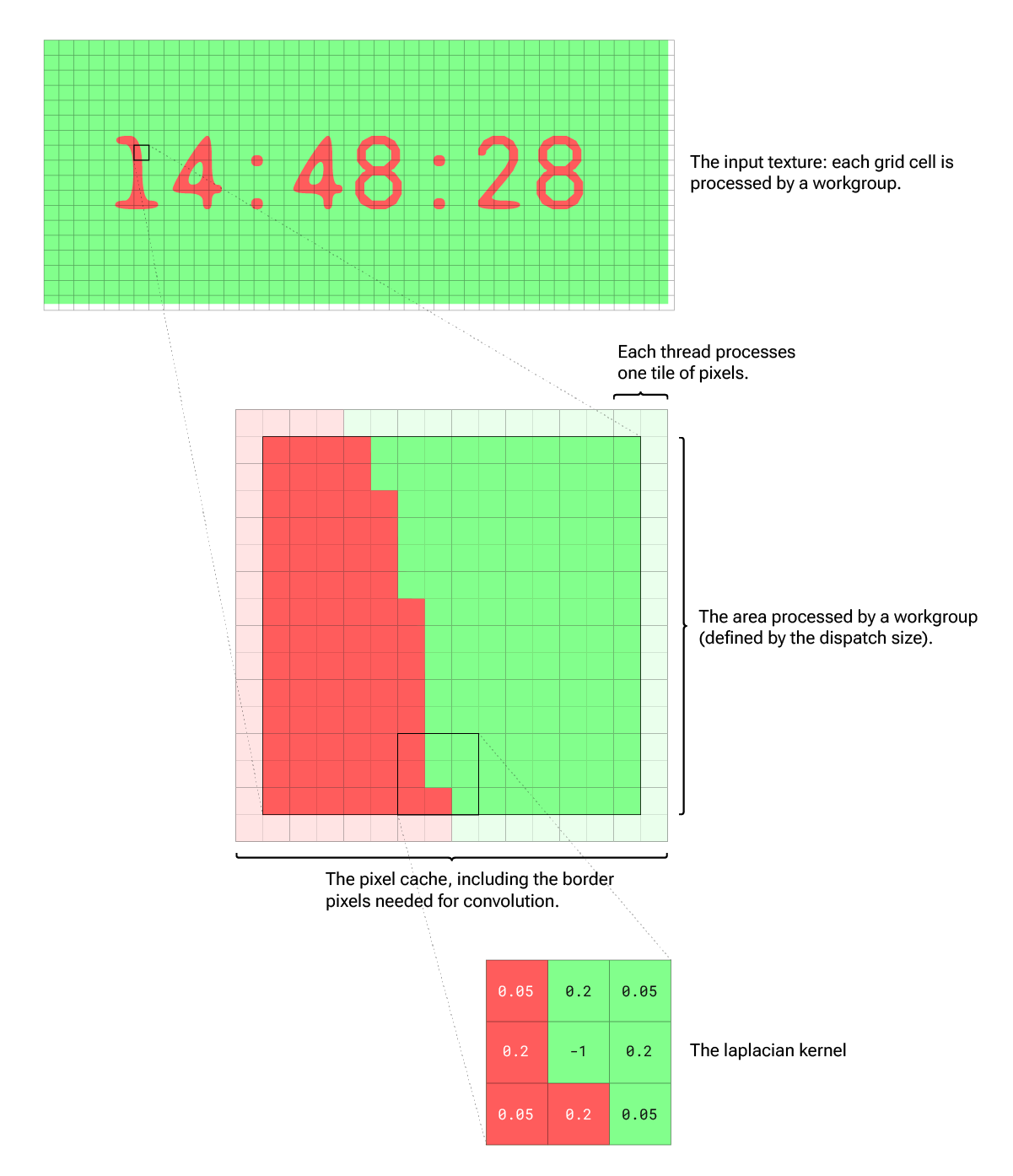
To make each workgroup cover a larger area (more pixels) we introduce a tile size. The tile size defines how many pixels each individual thread processes. This requires us to use a nested for loop within the shader, so we might want the keep the tile size very small (e.g., 2×2).
Pixel Cache
An essential step for running the reaction-diffusion simulation is the convolution with the laplacian kernel which is a 3×3 matrix. So, for each pixel we process, we have to read all 9 pixels that the kernel covers in order to perform the calculation. Due to the kernel overlap from pixel to pixel, there will be a lot of redundant texture reads.
Fortunately, compute shaders allow us to share memory across threads. So we can create what I call a pixel cache. The idea (from the image blur sample) is that each thread reads the pixels of its tile and writes them to the cache. Once every thread of the workgroup has stored its pixels in the cache (we ensure this with a workgroup barrier), the actual processing only needs to use the prefetched pixels from the cache. Hence it doesn’t require any further texture reads. The structure of the compute function might look something like this:
// the pixel cache shared accross all threads of the workgroup
var<workgroup> cache: array<array<vec4f, 128>, 128>;

@compute @workgroup_size(8, 8, 1)
fn compute_main(/* ...builtin variables */ ) {

  // add the pixels of this thread's tiles to the cache
  for (var c=0u; c<2; c++) {
    for (var r=0u; r<2; r++) {
      // ... calculate the pixel coords from the builtin variables
      // store the pixel value in the cache
      cache[y][x] = value;
    }
  }

  // don't continue until all threads have reached this point
  workgroupBarrier();

  // process every pixel of this threads tile
  for (var c=0u; c<2; c++) {
    for (var r=0u; r<2; r++) {
        // ...perform reaction-diffusion algorithm
        textureStore(/* ... */);
      }
    }
  }
}
But there’s another tricky aspect we have to watch out for: the kernel convolution requires us to read more pixels than we ultimately process. We could extend the pixel cache size. However, the size of the memory shared by the threads of a workgroup is limited to 16,384 bytes. Therefore we have to decrease the dispatch size by (kernelSize - 1)/2 on each side. Hopefully the following illustration will make these steps clearer.

UV Distortion
One disadvantage of using the compute shader compared to the fragment shader solution is that you cannot use a sampler for the storage textures within a compute shader (you can only load integer pixel coordinates). If you want to animate the simulation by moving the texture space (i.e., distorting the UV coordinates in fractional increments), you have to do the sampling yourself.
One way to deal with this is to use a manual bilinear sampling function. The sampling function used in the demo is based on the one shown here, with some adjustments for use within a compute shader. This allows us to sample fractional pixel values:
fn texture2D_bilinear(t: texture_2d<f32>, coord: vec2f, dims: vec2u) -> vec4f {
    let f: vec2f = fract(coord);
    let sample: vec2u = vec2u(coord + (0.5 - f));
    let tl: vec4f = textureLoad(t, clamp(sample, vec2u(1, 1), dims), 0);
    let tr: vec4f = textureLoad(t, clamp(sample + vec2u(1, 0), vec2u(1, 1), dims), 0);
    let bl: vec4f = textureLoad(t, clamp(sample + vec2u(0, 1), vec2u(1, 1), dims), 0);
    let br: vec4f = textureLoad(t, clamp(sample + vec2u(1, 1), vec2u(1, 1), dims), 0);
    let tA: vec4f = mix(tl, tr, f.x);
    let tB: vec4f = mix(bl, br, f.x);
    return mix(tA, tB, f.y);
}
This is how the pulsating movement of the simulation from the centre that can be seen in the demo was created.
Parameter Animation
One of the things I really like about reaction-diffusion is the variety of different patterns you can get by changing just a few parameters. If you then animate these changes over time or in response to user interaction, you can get really interesting effects. In the demo, for example, some parameters change depending on the distance from the centre or the speed of the pointer.
Composition Rendering
With the reaction-diffusion simulation done, the only thing left is to draw the result to the screen. This is the job of the composition render pipeline.
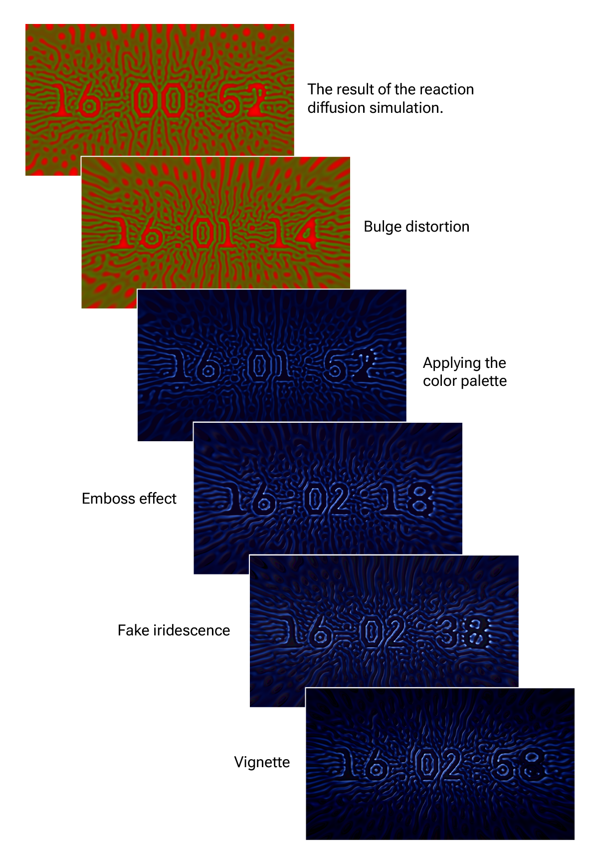
I just want to give a brief overview of the steps involved in the demo application. However, these depend very much on the style you want to achieve. Here are the main adjustments made during the composition pass of the demo:
- Bulge distortion: Before sampling the reaction-diffusion result texture, a bulge distortion is applied to the UV coordinates (based on this shadertoy code). This adds a sense of depth to the scene.
- Colour: A colour palette is applied (from Inigo Quilez)
- Emboss filter: A simple emboss effect gives the “veins” some volume.
- Fake iridescence: This subtle effect is based on a different colour palette, but is applied to the negative space of the embossing result. The fake iridescence makes the scene seem a little bit more vibrant.
- Vignette: A vignette overlay is used to darken the edges.

Conclusion
As far as performance is concerned, I have created a very basic performance test between a fragment variant and the compute variant (including bilinear sampling). At least on my device the compute variant is a lot faster. The performance tests are in a separate folder in the repository – only a flag in the main.js has to be changed to compare fragment with compute (GPU time measured with timestamp-query API).
I am still very new to WebGPU development. If anything in my tutorial can be improved or is not correct, I would be happy to hear about it.
Unfortunately, I couldn’t go into every detail and could only explain the idea behind using a compute shader for running a reaction-diffusion simulation very superficially. But I hope you enjoyed this tutorial and that you might be able to take a little something away with you for your own projects. Thanks for reading!

