

Want to learn how to discover and analyze the hidden patterns within your data? Clustering, an essential technique in Unsupervised Machine Learning, holds the key to discovering valuable insights that can revolutionize your understanding of complex datasets.
In this comprehensive handbook, we’ll delve into the must-know clustering algorithms and techniques, along with some theory to back it all up. Then you’ll see how it all works with plenty of examples, Python implementations, and visualizations.
Whether you’re a beginner or an experienced data scientist, this handbook is an invaluable resource for mastering clustering techniques. You can also download the handbook here.
If you enjoy learning through listening as well, here’s a 15-minute podcast where we discuss clustering in more detail. In this episode, we explore the fundamental concepts of clustering, providing a deeper understanding of how these techniques can be applied to real-world data.
Here’s what we’ll cover:
-
Introduction to Unsupervised Learning
-
Supervised vs. Unsupervised Learning
-
Important Terminology
-
How to Prepare Data for Unsupervised Learning
-
Clustering Explained
-
K-Means Clustering
-
Elbow Method for Optimal Number of Clusters (K)
-
Hierarchical Clustering
-
DBSCAN Clustering
-
How to Use t-SNE for Visualizing Clusters with Python
-
More Unsupervised Learning Techniques
By the end of this book, you’ll be able to:
-
Understand the fundamentals of Unsupervised Learning – You will grasp the key differences between supervised and unsupervised learning, and how clustering fits into the broader field of machine learning.
-
Master important clustering terminology – You will be familiar with essential concepts such as data points, centroids, distance metrics, and cluster evaluation methods.
-
Prepare data for clustering – You will learn how to handle missing values, normalize datasets, remove outliers, and apply dimensionality reduction techniques like PCA and t-SNE.
-
Gain a deep understanding of clustering techniques – You will explore various clustering methods, including K-Means, Hierarchical Clustering, and DBSCAN, and understand when to use each approach.
-
Implement K-Means clustering in Python – You will learn to apply the K-Means algorithm using Python, optimize the number of clusters with the Elbow Method, and visualize cluster results effectively.
-
Apply hierarchical clustering – You will understand Agglomerative and Divisive clustering, learn how to construct dendrograms, and use Python to implement hierarchical clustering.
-
Use DBSCAN for density-based clustering – You will master DBSCAN’s approach to clustering, including its ability to identify noise points and clusters of arbitrary shapes.
-
Visualize clustering results – You will be able to generate meaningful visualizations for clustering results using Matplotlib, Seaborn, and t-SNE to analyze and interpret data effectively.
-
Evaluate clustering performance – You will learn how to assess cluster quality using techniques like the Silhouette Score, Davies-Bouldin Index, and Calinski-Harabasz Index.
-
Work with real-world datasets – You will gain hands-on experience applying clustering techniques to real-world datasets, including customer segmentation, anomaly detection, and pattern recognition.
-
Expand your knowledge beyond clustering – You will be introduced to other unsupervised learning techniques, such as mixture models and topic modeling, broadening your expertise in machine learning.
By the end of this handbook, you will have a strong foundation in clustering and unsupervised learning, empowering you to analyze complex datasets and uncover hidden patterns with confidence!
Prerequisites
Before diving into this handbook on clustering and unsupervised learning, you should have a solid understanding of machine learning concepts, data preprocessing techniques, and basic Python programming skills. These prerequisites will help you grasp the theoretical foundations and practical implementations covered throughout the book.
First and foremost, it’s important to be familiar with machine learning fundamentals. You should understand the difference between supervised and unsupervised learning, as well as the core principles behind clustering techniques.
Concepts such as data points, features, distance metrics (Euclidean, Manhattan), and similarity measures play a significant role in clustering algorithms. A basic understanding of probability, statistics, and linear algebra will also be beneficial since these mathematical concepts form the foundation of many machine learning models.
Next, data preprocessing techniques are essential for working with real-world datasets. Since clustering algorithms rely heavily on well-structured data, you need to know how to handle missing values, normalize or standardize numerical features, and remove outliers that could distort clustering results.
Techniques like feature scaling (Min-Max normalization, Standardization) and dimensionality reduction (PCA, t-SNE) can improve clustering accuracy and efficiency, making it easier for you to interpret the results.
Finally, proficiency in Python programming and data science libraries is required to follow the hands-on implementations in this handbook. You should be comfortable working with libraries like NumPy and Pandas for data manipulation, Matplotlib and Seaborn for visualization, and Scikit-learn for implementing machine learning algorithms.
Since you’ll be applying clustering techniques such as K-Means, Hierarchical Clustering, and DBSCAN, familiarity with writing and executing Python scripts using Jupyter Notebooks, and interpreting clustering outputs, will enhance your learning experience.
By building a strong foundation in these areas, you’ll be well-prepared to unlock the power of clustering and gain deeper insights from your data.
Introduction to Unsupervised Learning
Unsupervised learning is a powerful technique in machine learning. It allows us to uncover hidden patterns and structures within data without any predefined labels or target variables. Unlike supervised learning, which relies on labeled data for training, unsupervised learning lets us explore and understand the inherent structure within unlabeled datasets.
One key application of unsupervised learning is clustering. Clustering is the process of grouping similar data points together based on their intrinsic characteristics and similarities. By identifying patterns and relationships within datasets, clustering helps us gain valuable insights and make sense of complex data.
Clustering finds its significance in various domains, including customer segmentation, anomaly detection, image recognition, and recommendation systems. It enables us to identify distinct groups within data, classify data into meaningful categories, and understand the underlying trends driving datasets.
In the next sections, we will delve deeper into different clustering algorithms, such as K-Means, hierarchical clustering, and DBSCAN, exploring their theories, implementations, and visualizations. By the end of this handbook, you will have a comprehensive understanding of unsupervised learning and be equipped with the knowledge and skills to apply various clustering techniques to your own data analysis tasks.
Remember, clustering is just one aspect of unsupervised learning, which offers a range of other techniques and applications. So, let’s dive in and discover the exciting world of unsupervised learning and the power it holds for extracting insights from unlabeled data.
Supervised vs. Unsupervised Learning
When it comes to machine learning, there are two primary approaches: supervised learning and unsupervised learning. Understanding the differences between these two approaches is crucial in selecting the right technique for your data analysis needs.
Supervised learning, as the name suggests, involves training a machine learning model on labeled data. In this approach, the input data consists of features (also known as attributes or variables) and corresponding target values or labels. The model learns from this labeled data and makes predictions or classifications based on new, unseen data.
On the other hand, unsupervised learning is all about exploring unlabeled data. With unsupervised learning, the data does not come with predefined labels or target values. Instead, the algorithm searches for patterns, structures, and relationships within the data on its own. The goal is to discover hidden insights and gain a deeper understanding of the underlying structure of the data.
One of the key advantages of unsupervised learning is its ability to uncover previously unknown patterns and relationships. Without the constraints of labeled data, unsupervised algorithms can reveal valuable insights that may not be apparent through other analytical methods. This makes unsupervised learning particularly useful in exploratory data analysis, anomaly detection, and clustering.
In supervised learning, the target variable serves as a guiding force for the learning process, enabling the model to make accurate predictions or classifications. But this reliance on labeled data can also limit the model’s capabilities, as it may struggle with unrepresented or novel patterns that were not present in the training data.
In contrast, unsupervised learning allows for a more flexible and adaptable approach. It can capture the underlying structure and relationships within the data, even when explicit labels are unavailable. By leveraging clustering algorithms and dimensionality reduction techniques, unsupervised learning offers powerful tools to unravel complex datasets.
In summary, supervised learning is well-suited for tasks where labeled data is available and the goal is to make precise predictions or classifications. Unsupervised learning, on the other hand, is valuable when exploring data for hidden patterns and relationships, especially in cases where labeled data is scarce or non-existent.
By understanding the differences between these two approaches, you can effectively choose the right technique to unleash the full potential of your data analysis efforts.
Important Terminology
To fully understand unsupervised learning and clustering, it’s crucial to be familiar with key terms associated with these concepts. Here are some important terminologies you should know:
1. Data Point
A data point refers to an individual observation or instance within a dataset. Each data point contains various features or attributes that describe a specific object or event.
2. Number of Clusters
The number of clusters represents the desired or estimated number of distinct groups in which the data will be partitioned during the clustering process. It is an essential parameter that determines the structure of the resulting clusters.
3. Unsupervised Algorithm
An unsupervised algorithm is a mathematical procedure used to identify patterns or relationships in data without the need for labeled or pre-categorized examples. These algorithms explore the inherent structure and complexity of datasets to uncover hidden insights.
Understanding and utilizing these terminologies will lay a strong foundation for your journey into unsupervised learning and clustering. In the following sections, we will delve deeper into the practical aspects and implementation of clustering techniques in Python.
How to Prepare Data for Unsupervised Learning
Before implementing unsupervised learning algorithms, it is crucial to ensure that the data is properly prepared. This involves taking certain steps to optimize the input data, making it suitable for analysis using clustering techniques. The following are important considerations when preparing data for unsupervised learning:
Data Normalization
One key aspect of data preparation is normalization, where all features are scaled to a consistent range. This is necessary because variables in the dataset may have different units or scales.
Normalization helps avoid bias towards any particular feature during the clustering process. Common methods for normalization include min-max scaling and standardization.
Handling Missing Values
Dealing with missing values is another critical step. It is important to identify and address any missing values in the dataset before applying clustering algorithms.
There are various techniques for handling missing values, such as imputation, where missing values are replaced with estimated values based on statistical methods or algorithms.
Outlier Detection and Treatment
Outliers can significantly impact clustering results, as they can influence the determination of cluster boundaries. So it’s essential to detect and handle outliers appropriately. This can involve techniques like Z-score or interquartile range (IQR) analysis to identify and treat outliers.
Dimensionality Reduction
In some cases, the dataset might have a high dimensionality, meaning it contains a large number of features. High-dimensional data can be challenging to visualize and analyze effectively. Dimensionality reduction techniques, such as Principal Component Analysis (PCA), can be employed to reduce the number of features while retaining the most informative aspects of the data.
By carefully preparing the data, normalizing variables, handling missing values, addressing outliers, and reducing dimensionality when necessary, you can optimize the quality of input data for unsupervised learning algorithms. This ensures accurate and meaningful clustering results, leading to valuable insights and patterns within the data.
Remember, data preparation is a crucial step in the unsupervised learning process, setting the foundation for successful clustering analysis.

Clustering Explained
Clustering is a fundamental technique in unsupervised learning that plays a crucial role in uncovering hidden patterns within data. It involves grouping data points based on their similarity, allowing us to identify distinct subsets or clusters within a dataset. By analyzing the structure of these clusters, we can gain valuable insights and make data-driven decisions.
Concept of Clustering
At its core, clustering aims to find similarities or relationships between data points without any predefined labels or target variables. The goal is to maximize the similarity within each cluster while maximizing the dissimilarity between different clusters. This process enables us to identify patterns and inherent structures within the data.
Clusters can be defined by various factors such as distance, connectivity, or density. Each data point within a cluster shares more similarities with other points in the same cluster than with points in other clusters. This grouping allows us to segment the data, which can be immensely useful in various domains such as customer segmentation, anomaly detection, and image recognition.
Types of Clustering Algorithms
There are several clustering algorithms available, each with its own approach to partitioning data into clusters. Some popular ones include K-Means Clustering, Hierarchical Clustering, and DBSCAN (Density-Based Spatial Clustering of Applications with Noise).
1. K-Means Clustering
K-Means Clustering is a widely used algorithm that aims to partition data into K distinct clusters. It iteratively assigns each data point to the nearest cluster centroid and then recomputes the centroids. This process continues until convergence, resulting in well-defined clusters.
2. Hierarchical Clustering
Hierarchical Clustering creates a hierarchy of clusters by recursively dividing or merging them based on certain criteria. This approach can be represented as a dendrogram, which provides valuable insights into the hierarchy and relationships between clusters.
3. DBSCAN Clustering
DBSCAN is a density-based algorithm that groups data points based on their density and connectivity. It is particularly effective in identifying clusters of arbitrary shapes and handling noisy data.
These are just a few examples of clustering algorithms, each with its own strengths and suitability for specific scenarios. It is important to select the most appropriate algorithm based on the data characteristics and problem domain.
In the next sections, we will delve deeper into the theories, implementation, and visualization of these clustering algorithms to provide you with a comprehensive understanding of how they work and when to use them.
Remember, clustering is a powerful technique that allows us to unlock the hidden structures within our data, leading to valuable insights and informed decision-making. Let’s dive into the world of clustering and discover the potential it holds.

K-Means Clustering
K-Means clustering is a popular unsupervised learning algorithm used to partition data points into distinct groups based on similarity. In this section, we will dive into the theory behind K-Means clustering and explore its implementation in Python using the scikit-learn library.
In Data Science and Data Analytics, we often want to categorize observations into set of segments or clusters for different purpose. For instance, a company might want to cluster its customers into 3–5 groups based on their transaction history or frequency of purchases. This is usually an Unsupervised Learning approach where the labels (groups/segments/clusters) are unknown.
One of the most popular clustering approaches for clustering observations into groups is the unsupervised clustering algorithm K-Means. Following are conditions for K-Means clustering:
-
number of clusters needs to be specified in advance: K
-
every observation needs to belong to at least one class
-
every observation need to belong to only one class (classes need to be non-overlapping)
-
no one observation should belong to more than 1 class
The idea behind K-Means is to minimize the within-cluster variation and maximize the between-cluster variation. So, for K-means to partition the observations into K clusters such that the total within-cluster variation, summed over all K clusters, is as small as possible.
The motivation behind this is to cluster observation so that the observations clustered to same group will be as similar as possible while the observations from different groups are as different as possible.
Mathematically, the within-cluster variation is defined based on the choice of distance measure which you can choose yourself. For instance, as distance measure you can use Euclidean distance, Manhattan distance etc.
K-means clustering is optimal when the within-cluster variation is the smallest. The within-cluster variation of C_k cluster is a measure W(C_k) of the amount by which the observations in a cluster differs from each other. So the following optimization problem should be solved:
$$\min_C_1, \dots, C_K \sum_k=1^K W(C_k)$$
Where within-cluster variation using Euclidean distance can be expressed as follows:
$$W(C_k) = \frac1C_k \sum_i,i’ \in C_k \sum_j=1^p (x_ij – x_i’j)^2$$
The number of observations in the kth cluster is denoted by |C_k |. Thus, the optimization problem for K-means can be described as follows:
$$\min_C_1, \dots, C_K \left\ \sum_k=1^K \frac1C_k \sum_i,i’ \in C_k \sum_j=1^p (x_ij – x_i’j)^2 \right\$$
K-Means Algorithm
The pseudocode of the K-means Algorithm can be described as follows:
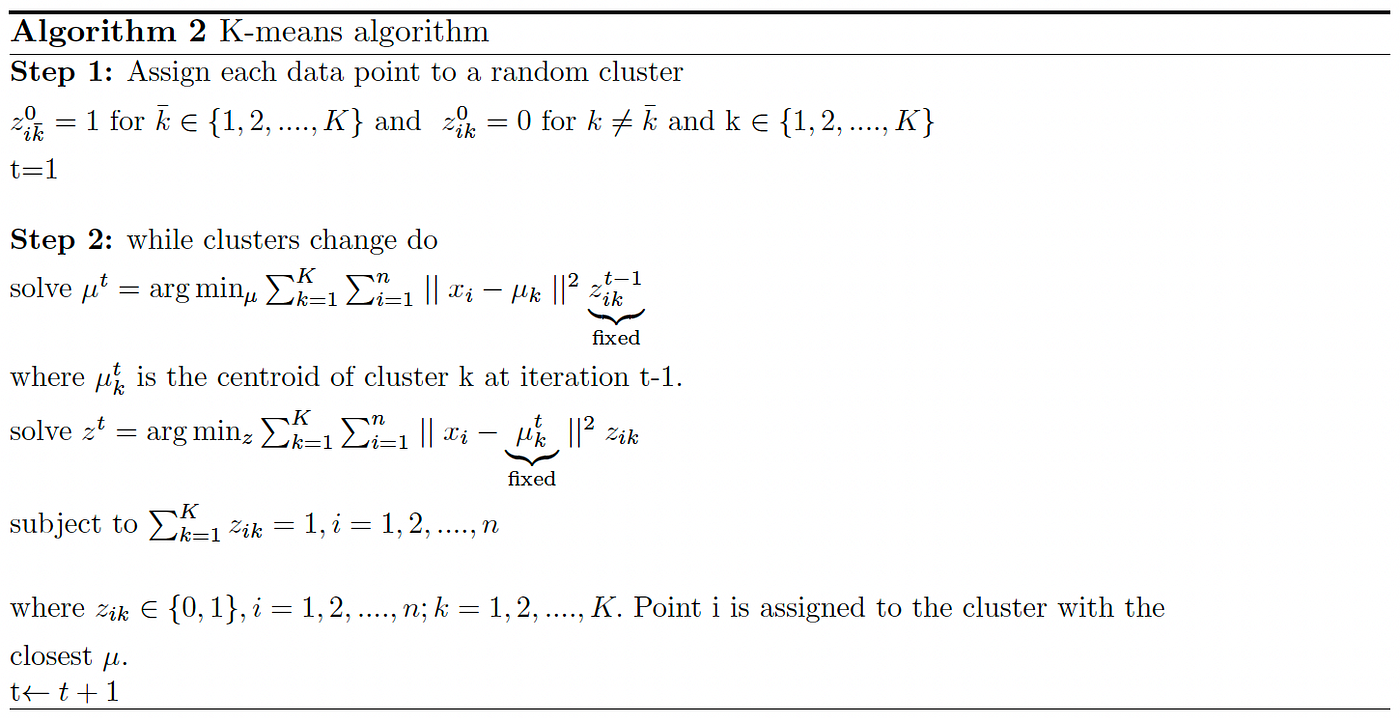
K-Means is a non-deterministic approach and it’s randomness comes in Step 1, where all observations are randomly assigned to 1 of the K classes.
In the second step, for each cluster, the cluster centroids are calculating by calculating the mean values of all the data points in the cluster. The centroid of a Kth cluster is a vector of length p containing the means of all variables for the observations in the kth cluster, and where p is the number of variables.
Then, in the next step, the clusters of observations are updated, such that each observation is assigned to a cluster where the centroid is the closest, by iteratively minimizing the total within sum of squares. That is, we iterate steps 2 and 3 until the cluster centroids are no longer changing or the maximum number of iterations is reached.
K-Means Clustering: Python Implementation
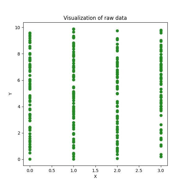
Let’s us look at an example where we aim to classify observations to 4 classes. The raw data looks like this:
from sklearn.cluster import KMeans

from sklearn import metrics

import numpy as np

import pandas as pd


df = np.random.randint(0, 10, size=[100, 2])

X1 = np.random.randint(0, 4, size=[300, 1])

X2 = np.random.uniform(0, 10, size=[300, 1])

df = np.append(X1, X2, axis=1)


Clustered_df = KMeans_Algorithm(df=df, K=4)

df = pd.DataFrame(Clustered_df)


def KMeans_Algorithm(df, K):
    """
    Perform K-Means clustering on the given dataset.

    Parameters:
    df (array-like): Input dataset to be clustered.
    K (int): Number of clusters.

    Returns:
    df (DataFrame): The original dataset with an additional column for cluster labels.
    """


    KMeans_model = KMeans(
        n_clusters=K,
        init='k-means++',
        max_iter=300,
        random_state=2021
    )


    KMeans_model.fit(df)


    centroids = KMeans_model.cluster_centers_


    centroids_df = pd.DataFrame(centroids, columns=["X", "Y"])


    labels = KMeans_model.labels_


    df = pd.DataFrame(df)


    df["labels"] = labels


    return d

This script is designed to generate synthetic data, apply K-Means clustering, and assign cluster labels to each data point. The K-Means clustering algorithm is an unsupervised machine learning method that groups similar data points into clusters based on their proximity in feature space. Below is a step-by-step breakdown of how the script works.
The first step is importing necessary libraries. The script uses KMeans from sklearn.cluster to implement the K-Means clustering algorithm. The metrics module from sklearn is included, though not used in this script, and can be helpful for evaluating clustering quality. NumPy is used for numerical computations and array operations, while Pandas is used to structure the data into a DataFrame for easier manipulation.
Next, the script generates synthetic numerical data. A NumPy array df is created with dimensions 100×2 containing random integers between 0 and 9. Two additional arrays, X1 and X2, are generated separately. X1 contains 300×1 random integers ranging from 0 to 3, and X2 contains 300×1 random floating-point numbers between 0 and 10. These arrays are then combined along the second axis to form a dataset with two features, making it ready for clustering.
Once the synthetic data is prepared, the script applies the K-Means clustering algorithm. The KMeans_Algorithm function is called with K=4, meaning the algorithm will attempt to group the data into four clusters. The function returns the clustered dataset, which is then converted into a Pandas DataFrame.
The KMeans_Algorithm function takes two parameters: the dataset df and the number of clusters K. Inside this function, the K-Means model is initialized using KMeans(). The number of clusters is set to K, and the init="k-means++" parameter ensures better initialization for faster convergence. The max_iter=300 argument sets a limit on the number of iterations, preventing excessive computation time. The random_state=2021 ensures that results are reproducible.
After initialization, the K-Means model is fitted to the dataset using KMeans_model.fit(df). This step processes the dataset, identifying cluster centers and grouping data points accordingly. Once training is complete, the cluster centroids are extracted using KMeans_model.cluster_centers_, and these are stored in a Pandas DataFrame with column names “X” and “Y” for easier interpretation.
Each data point is assigned a cluster label, which can be retrieved using KMeans_model.labels_. The script then ensures that the dataset is stored as a Pandas DataFrame, if not already formatted as one, and a new column "labels" is added to store the assigned cluster labels. Finally, the updated dataset, now containing the original features along with the cluster assignments, is returned.
The output of this script is a Pandas DataFrame containing three columns: two numerical feature columns representing the generated data points and one "labels" column that indicates the cluster assignment for each data point. For example, a simplified view of the output might show a row where a point with values [2.0, 7.4] is assigned to cluster 0, while another with [1.0, 3.2] belongs to cluster 1.
This script successfully creates a structured dataset, clusters the data into four distinct groups, and assigns meaningful cluster labels to each point. The results can be further analyzed through visualization techniques such as scatter plots to understand the clustering distribution. Future improvements might include using metrics like the Silhouette Score to evaluate clustering quality or experimenting with different numbers of clusters to find the most optimal grouping.
K-Means Clustering: Visualization
One of the key advantages of K-Means is its simplicity and efficiency in handling large datasets. It is a widely used clustering algorithm in various domains, including customer segmentation, image compression, anomaly detection, and pattern recognition.
Despite its simplicity, K-Means is highly effective in discovering inherent group structures within data, making it an essential tool in unsupervised learning. But like any algorithm, it has its limitations—such as sensitivity to the initial choice of centroids and difficulty in detecting non-spherical clusters. Understanding these strengths and weaknesses will help in making informed decisions when applying K-Means to real-world datasets.
In this section, we will explore how to implement K-Means clustering in Python and visualize the results. Through step-by-step code implementation, you will see how data points are grouped into clusters and how the algorithm iteratively refines its cluster assignments. We will also discuss best practices for selecting the optimal number of clusters and how to evaluate the clustering quality.
Understanding the K-Means Algorithm
Before we dive into the implementation, let’s briefly understand how the K-Means algorithm works. The algorithm follows these steps:
-
Step 1: Initialization – Randomly select K centroids, where K represents the desired number of clusters.
-
Step 2: Assignment – Assign each data point to the nearest centroid based on the Euclidean distance.
-
Step 3: Update – Recalculate the centroids by taking the mean of all data points assigned to each cluster.
-
Step 4: Repeat – Repeat steps 2 and 3 until convergence criteria are met (e.g., minimal centroid movement).
fig, ax = plt.subplots(figsize=(6, 6))


plt.scatter(df[df["labels"] == 0][0], df[df["labels"] == 0][1],
c='black', label='cluster 1')
plt.scatter(df[df["labels"] == 1][0], df[df["labels"] == 1][1],
c='green', label='cluster 2')
plt.scatter(df[df["labels"] == 2][0], df[df["labels"] == 2][1],
c='red', label='cluster 3')
plt.scatter(df[df["labels"] == 3][0], df[df["labels"] == 3][1],
c='y', label='cluster 4')
plt.scatter(centroids[:, 0], centroids[:, 1], marker='*', s=300, c='black', label='centroid')
plt.legend()
plt.xlim([-2, 6])
plt.ylim([0, 10])
plt.xlabel('X')
plt.ylabel('Y')
plt.title('Visualization of clustered data')
ax.set_aspect('equal')
plt.show()

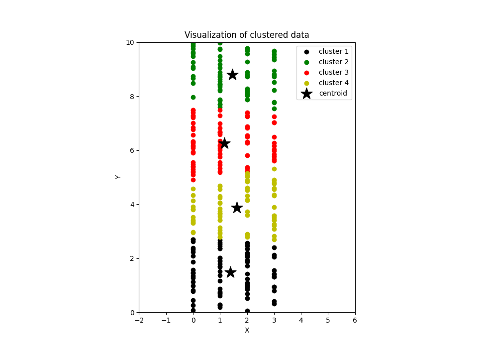
In the figure above, K-means has clustered these observations into 4 groups. And as you can see from the visualisation, the way observations have been clustered even by the graph seems natural and it makes sense.
Elbow Method for Optimal Number of Clusters (K)
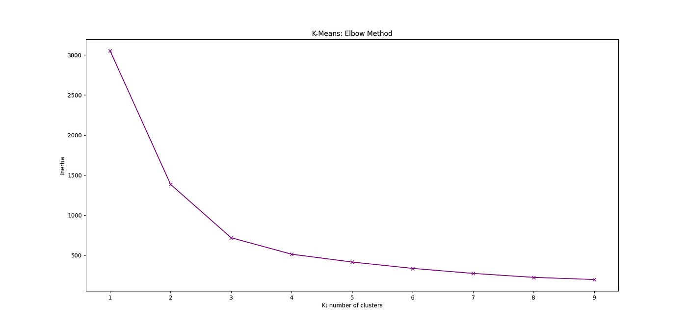
One of the biggest challenges in using K-means is the choice of clusters. Sometimes this is a business decision, but most of the time we want to pick a K that is optimal and makes sense. One of the most popular methods to determine this optimal value of K, or number of clusters, is the Elbow Method.
To use this approach, you need to know what Inertia is. Inertia is the sum of squared distances of samples to their closest cluster center. So, the Inertia or within cluster of sum of squares value gives an indication of how coherent the different clusters are or how pure they are. Inertia can be described as follows:
$$\sum_i=1^N (x_i – C_k)^2$$
where N is the number of samples within the data set, C is the centre of a cluster, and k is the cluster index. So, the Inertia simply computes the squared distance of each sample in a cluster to its cluster centre and sums them up.
Then we can calculate the inertia for different number of clusters K. We can plot this as in the following figure where we consider K = 1,2,….,10. Then from thee graph we can select the K corresponding to the Inertia where the elbow occurs. In this case, K = 3 where the Elbow happens.
def Elbow_Method(df):
    inertia = []

    K = range(1, 10)
    for k in K:
        KMeans_Model = KMeans(n_clusters=k, random_state = 2022)
        KMeans_Model.fit(df)
        inertia.append(KMeans_Model.inertia_)
    return(inertia)

K = range(1, 10)
inertia = Elbow_Method(df)
plt.figure(figsize = (17,8))
plt.plot(K, inertia, 'bx-')
plt.xlabel("K: number of clusters")
plt.ylabel("Inertia")
plt.title("K-Means: Elbow Method")
plt.show()

K-Means is a non-deterministic approach and it’s randomness comes in Step 1, where all observations are randomly assigned to 1 of the K classes.
So as you can see, K-Means clustering offers an efficient and effective approach to grouping data points based on similarity. By implementing the K-Means algorithm in Python, you can easily apply this technique to your own datasets and gain valuable insights into your data.
Python provides powerful tools for implementing and visualizing K-Means clustering. With the scikit-learn library and matplotlib, you can easily apply K-Means to your datasets and learn a lot from the resulting clusters.
Hierarchical Clustering Theory
Another popular clustering technique is Hierarchical Clustering. This is another unsupervised learning technique that helps us cluster observations into segments. But unlike of K-means, Hierarchical Clustering starts by treating each observation as a separate cluster.
Agglomerative vs. Divisive Clustering
There are two main types of hierarchical clustering: agglomerative and divisive.
Agglomerative clustering starts by assigning each data point to its own cluster. Then, it iteratively merges the most similar clusters based on a chosen distance metric until a single cluster containing all data points is formed.
This bottom-up approach creates a binary tree-like structure, also known as a dendrogram, where the height of each node represents the dissimilarity between the clusters being merged.
On the other hand, divisive clustering begins with a single cluster containing all data points. It then recursively divides the cluster into smaller subclusters until each data point is in its own cluster. This top-down approach generates a dendrogram that provides insights into the hierarchy of clusters.
Distance Metrics for Hierarchical Clustering
To determine the similarity between clusters or data points, there are various distance metrics you can use. Commonly employed distance measures include Euclidean distance, Manhattan distance, and cosine similarity. These metrics quantify the dissimilarity or similarity between pairs of data points and guide the clustering process.
In this technique, initially each data point is considered as an individual cluster. At each iteration, the most similar or the least dissimilar clusters merge into one cluster and this process continues until there is only a single cluster. So, the algorithm repeatedly performs the following steps:
-
1: identify the two clusters that are closest together
-
2: merge the two most similar clusters.
-
Then it continues this iterative process until all the clusters are merged together.
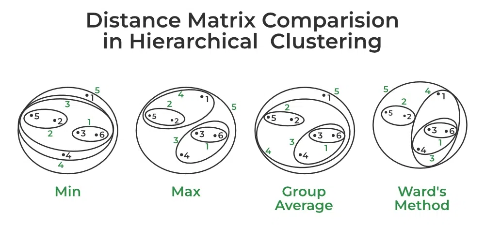
The dissimilarity or similarity of two clusters calculation depends on the Linkage type we assume. There are 5 popular linkage options:
-
Complete Linkage: max intercluster dissimilarity for which you need to compute all pairwise dissimilarities between the observations in cluster K1 and the observations in cluster K2. Then pick the largest of these similarities.
-
Single Linkage: min intercluster dissimilarity for which you need to compute all pairwise dissimilarities between the observations in cluster K1 and the observations in cluster K2. Then pick the smallest of these similarities.
-
Average Linkage: mean intercluster dissimilarity for which you need to compute all pairwise dissimilarities between the observations in cluster K1 and the observations in cluster K2. Then calculate the average of these similarities.
-
Centroid Linkage: dissimilarity between the centroid of cluster K1 and centroid of cluster K2 (this is usually the less desired choice of linkage since it might result in a lot of overlap).
-
Ward’s method: work out which observations to cluster based on reducing the sum of squared distances of each observation from the average observation in a cluster.
Hierarchical Clustering Python Implementation
Hierarchical clustering is a powerful unsupervised learning technique that allows you to group data points into clusters based on their similarity. In this section, we will explore the implementation of hierarchical clustering using Python.
Here is an example of how to implement hierarchical clustering using Python:
import scipy.cluster.hierarchy as HieraarchicalClustering
from sklearn.cluster import AgglomerativeClustering
import numpy as np
import pandas as pd


df = np.random.randint(0,10,size = [100,2])
X1 = np.random.randint(0,4,size = [300,1])
X2 = np.random.uniform(0,10,size = [300,1])
df = np.append(X1,X2,axis = 1)
hierCl = HieraarchicalClustering.linkage(df, method='ward')

Hcl= AgglomerativeClustering(n_clusters = 7, affinity = 'euclidean', linkage ='ward')
Hcl_fitted = Hcl.fit_predict(df)
df = pd.DataFrame(df)
df["labels"] = Hcl_fitted

This code implements hierarchical clustering using both Scipy’s hierarchical clustering module and Scikit-learn’s Agglomerative Clustering algorithm. The purpose of the script is to generate a synthetic dataset, apply hierarchical clustering, and assign cluster labels to the data points.
The first part of the script imports the necessary libraries. Scipy’s hierarchical clustering module (scipy.cluster.hierarchy) is imported as HieraarchicalClustering, which is used to perform linkage-based clustering. The AgglomerativeClustering class from Scikit-learn is also imported to implement a specific type of hierarchical clustering. Also, NumPy is used for numerical operations and generating random data, while Pandas is used to structure the data into a DataFrame.
Next, the script generates synthetic numerical data. A 100×2 matrix (df) is created with random integers between 0 and 9. Then, two additional datasets, X1 and X2, are created separately. X1 contains 300 random integers between 0 and 3, while X2 contains 300 random floating-point values between 0 and 10. These two datasets are then combined along the second axis using np.append(), forming a dataset with two features that will be used for clustering.
Once the dataset is prepared, hierarchical clustering is applied using the Ward linkage method, which minimizes the variance between merged clusters. The linkage matrix hierCl is created using HieraarchicalClustering.linkage(df, method='ward'), which computes the hierarchical clustering solution.
After generating the hierarchical clustering linkage matrix, Agglomerative Clustering is applied to group the data into seven clusters (n_clusters=7). The affinity='euclidean' parameter specifies that Euclidean distance will be used as the distance metric to measure similarity between points. The linkage="ward" parameter ensures that Ward’s method is used to merge clusters based on minimizing variance. The model is then fitted to the dataset using Hcl.fit_predict(df), which assigns a cluster label to each data point.
Finally, the dataset is converted into a Pandas DataFrame, and a new column "labels" is added to store the assigned cluster labels. The resulting DataFrame now contains both the original data points and their corresponding cluster assignments, allowing for further analysis or visualization.
In summary, this script generates random data, applies hierarchical clustering using both Scipy’s linkage method and Scikit-learn’s Agglomerative Clustering, and assigns cluster labels to each data point. The final dataset can be used to analyze cluster structures, visualize results, or validate clustering effectiveness.
Hierarchical Clustering: Visualization
One of the key advantages of hierarchical clustering is its ability to create a hierarchical structure of clusters, which can provide valuable insights into the relationships between data points.
To visualize hierarchical clustering in Python, we can use various libraries such as Scikit-learn, SciPy, and Matplotlib. These libraries offer easy-to-use functions and tools that facilitate the visualization process.
So, after performing hierarchical clustering, it is often helpful to visualize the clusters. We can use various techniques for visualization, such as dendrograms or heatmaps.
As we discussed above, a dendrogram is a tree-like diagram that shows the hierarchical relationships between clusters. It can be generated using the Scipy library in Python.
Here is an example of how to visualize a dendogram and clustered points in Python:
dendrogram = HieraarchicalClustering.dendrogram(hierCl)
plt.title('Dendrogram')
plt.xlabel("Observations")
plt.ylabel('Euclidean distances')
plt.show()
plt.scatter(df[df["labels"] == 0][0], df[df["labels"] == 0][1],
c='black', label='cluster 1')
plt.scatter(df[df["labels"] == 1][0], df[df["labels"] == 1][1],
c='green', label='cluster 2')
plt.scatter(df[df["labels"] == 2][0], df[df["labels"] == 2][1],
c='red', label='cluster 3')
plt.scatter(df[df["labels"] == 3][0], df[df["labels"] == 3][1],
c='magenta', label='cluster 4')
plt.scatter(df[df["labels"] == 4][0], df[df["labels"] == 4][1],
c='purple', label='cluster 5')
plt.scatter(df[df["labels"] == 5][0], df[df["labels"] == 5][1],
c='y', label='cluster 6')
plt.scatter(df[df["labels"] == 6][0], df[df["labels"] == 6][1],
c='black', label='cluster 7')
plt.legend()
plt.xlabel('X')
plt.ylabel('Y')
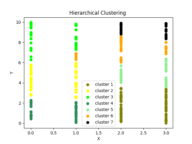
plt.title('Hierarchical Clustering')
plt.show()

Here is a step-by-step guide to visualizing hierarchical clustering in Python:
Step 1: Preprocess the data
Before visualizing hierarchical clustering, it is important to preprocess the data by scaling or normalizing it. This ensures that all features have a similar range and prevents any bias towards specific features.
Step 2: Perform hierarchical clustering
Next, we perform hierarchical clustering using the chosen algorithm, such as AgglomerativeClustering from Scikit-learn. This algorithm calculates the similarity between data points and merges them into clusters based on a specific linkage criterion.
Step 3: Create a dendrogram
We can use the dendrogram function from the SciPy library to create this visualization. The dendrogram allows us to visualize the distances and relationships between clusters.
Step 4: Plot the clusters
Finally, we can plot the clusters using a scatter plot or another suitable visualization technique. This helps us visualize the data points within each cluster and gain insights into the characteristics of each cluster.
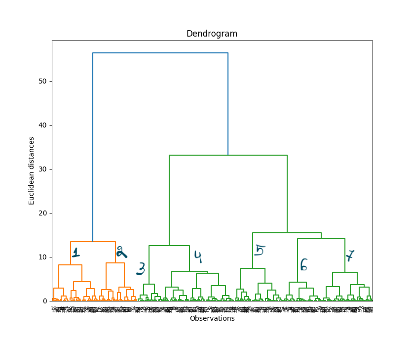
This dendogram can then help us to decide the number of clusters we can better use. As you can see, it seems like, in this case, we should use 7 clusters.
By visualizing hierarchical clustering in Python, we can gain a better understanding of the structure and relationships within our data. This visualization technique is particularly useful when dealing with complex datasets and can assist in decision-making processes and pattern discovery.
Remember to adjust the specific parameters and settings based on your dataset and objective. Experimenting with different visualizations and techniques can lead to even deeper insights into your data.
DBSCAN Clustering Theory
DBSCAN (Density-Based Spatial Clustering of Applications with Noise) is an unsupervised learning algorithm used for clustering analysis. It’s particularly effective in identifying clusters of arbitrary shape and handling noisy data.
Unlike K-Means or Hierarchical clustering, DBSCAN does not require specifying the number of clusters in advance. Instead, it defines clusters based on density and connectivity within the data.
How DBSCAN Works:
Density-Based Clustering: DBSCAN groups data points together that are in close proximity to each other and have a sufficient number of nearby neighbors. It identifies dense regions of data points as clusters and separates sparse regions as noise.
Core Points, Border Points, and Noise Points: DBSCAN categorizes data points into three types: Core Points, Border Points, and Noise Points.
-
Core Points: Data points with a minimum number of neighboring points (defined by the
min_samplesparameter) within a specified distance (defined by theepsparameter). -
Border Points: Data points that are within the
epsdistance of a Core Point but do not have enough neighboring points to be considered Core Points. -
Noise Points: Data points that are neither Core Points nor Border Points.
Reachability and Connectivity: DBSCAN uses the notions of reachability and connectivity to define clusters. A data point is considered reachable from another data point if there is a path of Core Points that connects them. If two data points are reachable, they belong to the same cluster.
Cluster Growth: DBSCAN starts with an arbitrary data point and expands the cluster by examining its neighbors and their neighbors, forming a connected group of data points.
Benefits of DBSCAN Clustering:
-
Ability to detect complex structures: DBSCAN can discover clusters of various shapes and sizes, making it well-suited for datasets with non-linear relationships or irregular patterns.
-
Robust to noise: DBSCAN handles noisy data effectively by categorizing noise points separately from clusters.
-
Automatic determination of cluster numbers: DBSCAN does not require specifying the number of clusters in advance, making it more convenient and adaptable to different datasets.
-
Scaling to large datasets: DBSCAN’s time complexity is relatively low compared to some other clustering algorithms, allowing it to scale well to large datasets.
In the next section, we will delve into the implementation of the DBSCAN algorithm in Python, providing step-by-step guidance and examples.
DBSCAN Clustering: Python Implementation
In this section, I’ll guide you through how to implement DBSCAN using Python.
Key Steps for DBSCAN Clustering
-
Prepare the data: Before applying DBSCAN, it is important to preprocess your data. This includes handling missing values, normalizing features, and selecting the appropriate distance metric.
-
Define the parameters: DBSCAN requires two main parameters: epsilon (ε) and minimum points (MinPts). Epsilon determines the maximum distance between two points to consider them as neighbors, and MinPts specifies the minimum number of points required to form a dense region.
-
Perform density-based clustering: DBSCAN starts by randomly selecting a data point and identifying its neighbors within the specified epsilon distance. If the number of neighbors exceeds the MinPts threshold, a new cluster is formed. The algorithm expands this cluster by iteratively adding new points until no more points can be reached.
-
Perform noise detection: Points that do not belong to any cluster are considered as noise or outliers. These points are not assigned to any cluster and can be critical in identifying anomalies within the data.
To perform DBSCAN clustering in Python, we can use the scikit-learn library. The first step is to import the necessary libraries and load the dataset we want to cluster. Then, we can create an instance of the DBSCAN class and set the epsilon (eps) and minimum number of samples (min_samples) parameters.
Here is a sample code snippet to get you started:
import numpy as np
import matplotlib.pyplot as plt
from sklearn.datasets import make_moons
from sklearn.cluster import DBSCAN


X, _ = make_moons(n_samples=500, noise=0.05, random_state=0)


db = DBSCAN(eps=0.3, min_samples=5, metric='euclidean')
y_db = db.fit_predict(X)

Remember to replace X with your actual data set. You can adjust the eps and min_samples parameters to get different clustering results. The eps parameter is the maximum distance between two samples for one to be considered as in the neighborhood of the other. The min_samples is the number of samples (or total weight) in a neighborhood for a point to be considered as a core point.
DBSCAN offers various advantages over other clustering algorithms, like not requiring the number of clusters to be predefined. This makes it suitable for data sets with an unknown number of clusters. DBSCAN is also capable of identifying clusters of varying shapes and sizes, making it more flexible in capturing complex structures.
But DBSCAN may struggle with varying densities in data sets and can be sensitive to the choice of epsilon and minimum points parameters. It is crucial to fine-tune these parameters to obtain optimal clustering results.
By implementing DBSCAN in Python, you can leverage this powerful clustering algorithm to uncover meaningful patterns and structures in your data.
Before we explore the differences between DBSCAN and other clustering techniques, let’s take a closer look at the key parameters that influence DBSCAN’s performance and results.
Understanding Key Parameters in DBSCAN
The eps (epsilon) parameter defines the maximum distance between two points for one to be considered as a neighbor of the other. This means that points within this radius of a core point belong to the same cluster. Choosing an appropriate eps value is crucial, as a very small eps may lead to too many small clusters, while a very large eps could merge distinct clusters into one.
The min_samples parameter determines the minimum number of data points required to form a dense region. If a point has at least min_samples neighbors within the eps radius, it is classified as a core point. If a point falls within the eps radius of a core point but does not meet the min_samples threshold itself, it is classified as a border point. Any point that is neither a core point nor a border point is labeled as noise or an outlier.
How DBSCAN Groups Data Points
DBSCAN operates by identifying core points and expanding clusters around them. It groups together closely packed points (or clusters) based on density and marks low-density points as outliers (or noise). The process follows these steps:
-
Select an unvisited point and check if it has at least
min_samplesneighbors within theepsradius. -
If it does, this point becomes a core point, and a new cluster is formed around it.
-
Expand the cluster by adding all directly reachable points within
eps. If any of these points are also core points, their neighbors are added as well. -
Continue expanding until no more points meet the density criteria.
-
Move to the next unvisited point and repeat the process.
-
Classify remaining points as border points (part of a cluster but not core points) or noise (outliers that do not belong to any cluster).
Example Implementation of DBSCAN
In this implementation:
-
eps=0.3: Defines how close points should be to be considered neighbors. -
min_samples=5: Sets the minimum number of points required to form a dense region. -
fit_predict(X): Assigns a cluster label to each data point.
After applying DBSCAN, the data points are assigned labels. If two points belong to the same cluster, they will have the same label in y_db. Points identified as outliers will be labeled as -1 and remain unclustered.
The resulting scatter plot visually represents how DBSCAN has identified two moon-shaped clusters. Unlike K-Means, which assumes spherical clusters, DBSCAN is able to detect arbitrary-shaped clusters effectively.
plt.scatter(X[y_db == 0, 0], X[y_db == 0, 1],
            c='lightblue', marker='o', s=40,
            edgecolor='black',
            label='cluster 1')
plt.scatter(X[y_db == 1, 0], X[y_db == 1, 1],
            c='red', marker='s', s=40,
            edgecolor='black',
            label='cluster 2')
plt.legend()
plt.show()

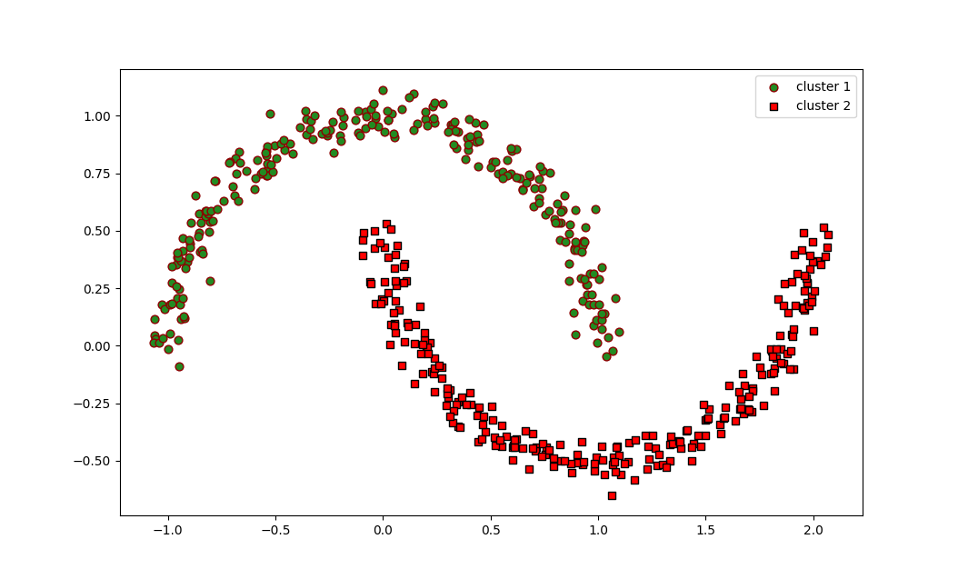
The resulting plot will show two moon-shaped clusters in green and red colors, demonstrating that DBSCAN successfully identified and separated the two interleaved half circles.
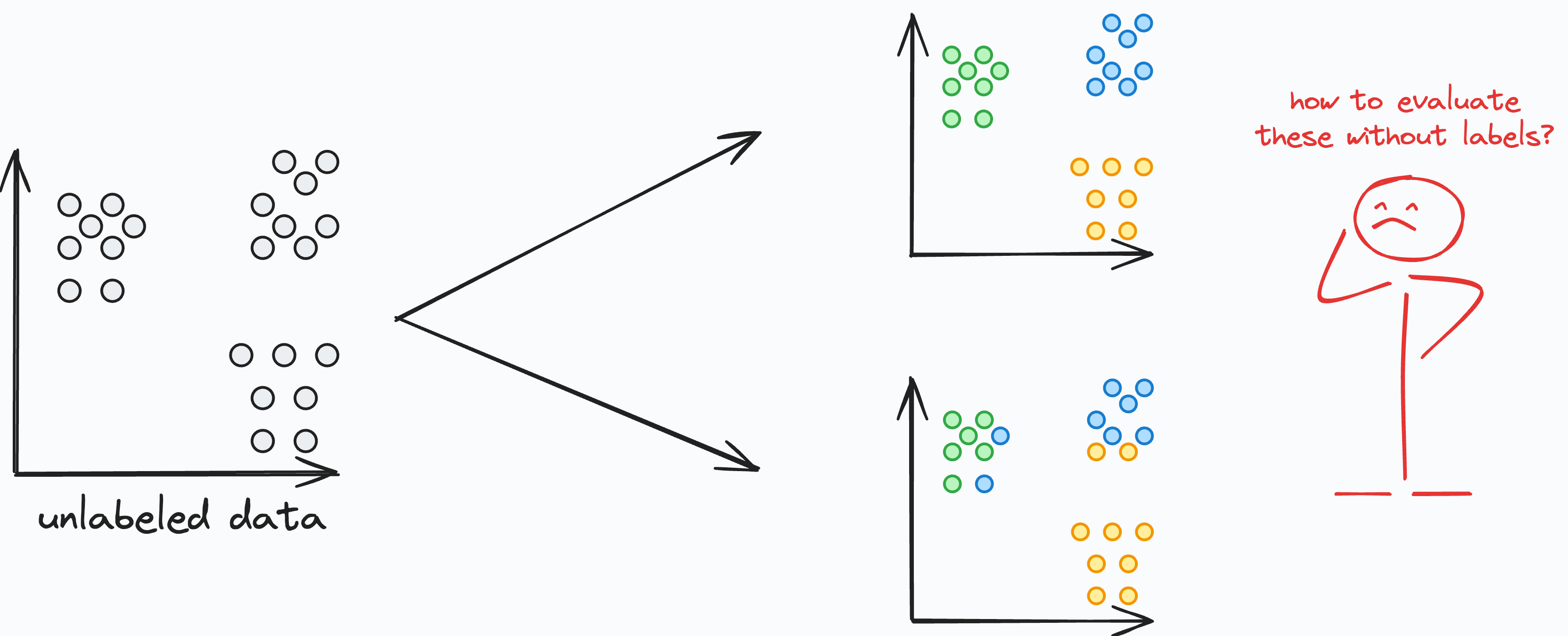
How to Evaluate the Performance of a Clustering Algorithm
Evaluating the performance of a clustering model can be challenging, as there are no ground truth labels available in unsupervised learning. But there are several evaluation metrics that can provide insights into the quality of the clustering results.
-
Silhouette coefficient: Measures how well each data point fits into its assigned cluster compared to other clusters. A higher silhouette coefficient indicates better clustering.
-
Davies-Bouldin index: Measures the average similarity between each cluster and its most similar cluster, while considering the separation between clusters. Lower values indicate better clustering.
-
Calinski-Harabasz index: Evaluates the ratio of between-cluster dispersion to within-cluster dispersion. Higher values indicate better-defined clusters.
-
Visual assessment: Inspecting visual representations of the clustering results, such as scatter plots or dendrograms, can also provide valuable insights into the quality and meaningfulness of the clusters.
I would recommended that you use a combination of evaluation metrics and visual assessments to comprehensively assess the performance of a clustering model.
Difference Between K-Means, Hierarchical Clustering, and DBSCAN
K-Means, Hierarchical Clustering, and DBSCAN are three widely used clustering algorithms, each with their own approach to grouping data points. Understanding their differences is crucial in selecting the most suitable method based on data characteristics and analytical objectives.
K-Means Clustering
K-Means clustering is a centroid-based algorithm that partitions data into K clusters based on similarity. The algorithm starts by randomly initializing K centroids and then iteratively assigns each data point to the nearest centroid. Once all data points are assigned, the centroids are recalculated based on the mean of the points within each cluster. This process continues until convergence is reached.
Strengths of K-Means Clustering:
-
Efficient and scalable for large datasets.
-
Works well when clusters are spherical and evenly distributed.
-
Computationally faster compared to hierarchical clustering.
-
Easy to implement and interpret.
Weaknesses of K-Means Clustering:
-
Requires specifying the number of clusters (K) in advance.
-
Sensitive to initial centroid positions, leading to varying results.
-
Assumes clusters are of equal size and spherical, which is not always the case.
-
Struggles with outliers and non-linear shaped clusters.
Hierarchical Clustering
Hierarchical clustering creates a nested hierarchy of clusters without requiring a predefined number of clusters. It starts by treating each data point as an individual cluster and progressively merges or splits clusters based on similarity. The results are often visualized using a dendrogram, which helps determine the optimal number of clusters.
Strengths of Hierarchical Clustering:
-
Does not require specifying the number of clusters in advance.
-
Captures hierarchical relationships between clusters.
-
Can handle different types of data, including numerical and categorical.
-
Useful for exploratory analysis with a dendrogram for better interpretability.
Weaknesses of Hierarchical Clustering:
-
Computationally expensive for large datasets (O(n²) complexity).
-
Hard to scale due to memory constraints when processing large numbers of data points.
-
Choosing the right cut-off point for the dendrogram can be challenging.
-
Sensitive to noise and outliers, which can distort the hierarchy.
DBSCAN (Density-Based Spatial Clustering of Applications with Noise)
DBSCAN is a density-based clustering algorithm that groups data points based on their proximity and density rather than predefined clusters. Unlike K-Means and Hierarchical Clustering, DBSCAN does not require specifying the number of clusters. Instead, it uses two key parameters: eps (the maximum distance between two points to be considered neighbors) and min_samples (the minimum number of points required to form a dense cluster). Points that do not meet these criteria are classified as noise.
Strengths of DBSCAN:
-
Does not require specifying the number of clusters in advance.
-
Can detect arbitrarily shaped clusters, unlike K-Means which assumes spherical clusters.
-
Effectively handles outliers, which are labeled as noise instead of forcing them into a cluster.
-
Suitable for datasets with varying densities and non-linear structures.
Weaknesses of DBSCAN:
-
Struggles with varying cluster densities, as a single eps value may not fit all clusters.
-
Can be sensitive to parameter tuning (eps and min_samples) which can impact clustering performance.
-
Not ideal for high-dimensional data, as Euclidean distance loses meaning in high-dimensional spaces.
-
May struggle with very large datasets, though it scales better than hierarchical clustering.
Choosing the Right Clustering Algorithm
| Feature | K-Means | Hierarchical Clustering | DBSCAN |
| Cluster Shape | Assumes spherical clusters | Works well with hierarchical structures | Handles arbitrary-shaped clusters |
| Scalability | Very scalable (fast for large datasets) | Not scalable (O(n²) complexity) | Moderately scalable (can struggle with very large datasets) |
| Number of Clusters | Must be predefined | No need to specify | No need to specify |
| Handling Outliers | Poor | Sensitive to noise | Good, detects outliers as noise |
| Computation Complexity | O(n) to O(n log n) | O(n²) | O(n log n) |
| Interpretability | Easy to interpret results | Dendrogram provides good insight | Less intuitive, requires parameter tuning |
Each clustering algorithm has its strengths and weaknesses. K-Means is ideal when dealing with large datasets and when clusters are spherical and well-separated. Hierarchical Clustering is useful when hierarchical relationships exist or when the number of clusters is unknown. DBSCAN excels in detecting arbitrarily shaped clusters and handling noise but requires careful tuning of parameters.
By understanding the characteristics of each algorithm, you can make an informed decision on which clustering method best suits your data analysis needs.
How to Use t-SNE for Visualizing Clusters with Python
After applying clustering algorithms like K-Means, Hierarchical Clustering, and DBSCAN, you’ll often want to visualize the resulting clusters to gain a better understanding of the underlying data structure.
While scatter plots work well for datasets with two or three dimensions, real-world datasets often contain high-dimensional features that are difficult to interpret visually.
To address this challenge, you can use dimensionality reduction techniques like t-SNE (t-Distributed Stochastic Neighbor Embedding) to project high-dimensional data into a lower-dimensional space while preserving its structure. This allows you to visualize clusters more effectively and identify hidden patterns that may not be immediately apparent in raw data.
In this section, we will explore the theory behind t-SNE and its implementation in Python.
Understanding t-SNE
t-SNE was introduced by Laurens van der Maaten and Geoffrey Hinton in 2008 as a method to visualize complex data structures. It aims to represent high-dimensional data points in a lower-dimensional space while preserving the local structure and pairwise similarities among the data points.
t-SNE achieves this by modeling the similarity between data points in the high-dimensional space and the low-dimensional space.
The t-SNE Algorithm
The t-SNE algorithm proceeds in the following steps:
-
Compute pairwise similarities between data points in the high-dimensional space. This is typically done using a Gaussian kernel to measure the similarity based on the Euclidean distances between data points.
-
Initialize the low-dimensional embedding randomly.
-
Define a cost function that represents the similarity between data points in the high-dimensional space and the low-dimensional space.
-
Optimize the cost function using gradient descent to minimize the divergence between the high-dimensional and low-dimensional similarities.
-
Iterate steps 3 and 4 until the cost function converges.
Implementing t-SNE in Python is relatively straightforward with the help of libraries such as scikit-learn. The scikit-learn library provides a user-friendly API for applying t-SNE to your data. By following the scikit-learn documentation and examples, you can easily incorporate t-SNE into your machine learning pipeline.
2D t-SNE Visualisation
import matplotlib.pyplot as plt
from sklearn import datasets
from sklearn.manifold import TSNE


digits = datasets.load_digits()
X, y = digits.data, digits.target


tsne = TSNE(n_components=2, random_state=0)
X_tsne = tsne.fit_transform(X)


plt.figure(figsize=(10, 6))
scatter = plt.scatter(X_tsne[:, 0], X_tsne[:, 1], c=y, edgecolor='none', alpha=0.7, cmap=plt.cm.get_cmap('jet', 10))
plt.colorbar(scatter)
plt.title("t-SNE of Digits Dataset")
plt.show()

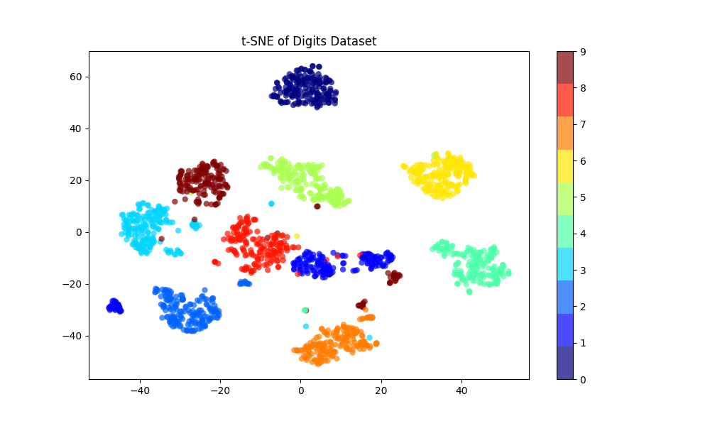
In this example:
-
We load the
digitsdataset. -
We apply t-SNE to reduce the data from 64 dimensions (since each image is 8×8) to 2 dimensions.
-
We then plot the transformed data, coloring each point by its true digit label.
The resulting visualization will show clusters, each corresponding to one of the digits (0 through 9). This helps to understand how well-separated the different digits are in the original high-dimensional space.
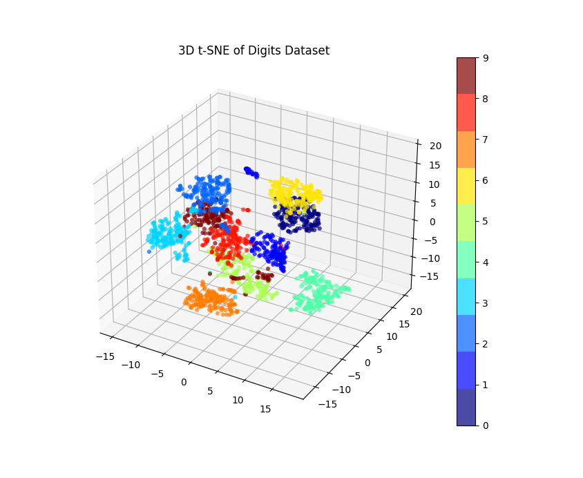
Visualizing High-Dimensional Data
One of the main advantages of t-SNE is its ability to visualize high-dimensional data in a lower-dimensional space. By reducing the dimensionality of the data, t-SNE enables us to identify clusters and patterns that may not be apparent in the original high-dimensional space. The resulting visualization can provide valuable insights into the structure of the data and aid in decision-making processes.
import matplotlib.pyplot as plt
from sklearn import datasets
from sklearn.manifold import TSNE
from mpl_toolkits.mplot3d import Axes3D


digits = datasets.load_digits()
X, y = digits.data, digits.target


tsne = TSNE(n_components=3, random_state=0)
X_tsne = tsne.fit_transform(X)


fig = plt.figure(figsize=(10, 8))
ax = fig.add_subplot(111, projection='3d')
scatter = ax.scatter(X_tsne[:, 0], X_tsne[:, 1], X_tsne[:, 2], c=y, edgecolor='none', alpha=0.7, cmap=plt.cm.get_cmap('jet', 10))
plt.colorbar(scatter)
plt.title("3D t-SNE of Digits Dataset")
plt.show()

In this revised code:
-
We set
n_components=3for t-SNE to get a 3D transformation. -
We use
mpl_toolkits.mplot3d.Axes3Dto create a 3D scatter plot.
After executing this code, you’ll see a 3D scatter plot where points are positioned based on their t-SNE coordinates, and they’re colored based on their true digit label.
Rotating the 3D visualization can help us understand the spatial distribution of the data points better.
t-SNE is a powerful tool for dimensionality reduction and visualization of high-dimensional data. By leveraging its capabilities, you can gain a deeper understanding of complex datasets and uncover hidden patterns that may not be immediately obvious. With its Python implementation and ease of use, t-SNE is a valuable asset for any data scientist or machine learning practitioner.
More Unsupervised Learning Techniques
In addition to the clustering techniques we’ve discussed here, there are some other important unsupervised learning techniques worth exploring. While we won’t delve into them in detail here, let’s briefly mention two of these techniques: mixture models and topic modeling.
Mixture Models
Mixture models are probabilistic models used for modeling complex data distributions. They assume that the overall dataset can be described as a combination of multiple underlying subpopulations or components, each described by its own probability distribution.
Mixture models can be particularly useful in situations where data points do not clearly belong to distinct clusters and may exhibit overlapping characteristics.
Topic Modeling
Topic modeling is a technique used to extract underlying themes or topics from a collection of documents. It allows you to explore and discover latent semantic patterns in text data.
By analyzing the co-occurrence of words across documents and identifying common themes, topic modeling enables automatic categorization and summarization of large textual datasets. This technique has applications in fields like natural language processing, information retrieval, and content recommendation systems.
While these techniques warrant further exploration beyond the scope of this handbook, they are valuable tools to consider for uncovering hidden patterns and gaining insights from your data.
Remember, mastering unsupervised learning involves continuous learning and practice. By familiarizing yourself with different techniques like the ones mentioned above, you’ll be well-equipped to tackle a wide range of data analysis problems across various domains.
FAQs
Q: What is the difference between supervised and unsupervised learning?
Supervised learning involves training a model on labeled data, where the inputs are paired with corresponding outputs. The goal is to predict the output for new, unseen inputs.
In contrast, unsupervised learning deals with unlabeled data, where the goal is to discover patterns, structures, or clusters within the data without any predefined output.
Essentially, supervised learning aims to learn a mapping function, while unsupervised learning focuses on uncovering hidden relationships or groupings in the data.
Q: Which clustering algorithm is best for my data?
The suitability of a clustering algorithm depends on various factors, such as the nature of the data, the desired number of clusters, and the specific problem you are trying to solve.
In this handbook, we discussed three commonly used clustering algorithms:
-
K-means is a popular algorithm that aims to partition the data into K clusters, with each data point assigned to the nearest centroid. It works well for evenly distributed, spherical clusters and requires the number of clusters to be specified in advance.
-
Hierarchical clustering builds a hierarchy of clusters by iteratively merging or splitting them. It provides a dendrogram to visualize the clustering process and can handle different shapes and sizes of clusters.
-
DBSCAN is a density-based algorithm that groups together data points that are close to each other and separates outliers. It can discover clusters of arbitrary shape and does not require the number of clusters to be known beforehand.
To determine the best algorithm for your use case, I recommend that you experiment with different techniques and assess their performance based on metrics like cluster quality, computational efficiency, and interpretability.
Q: Can unsupervised learning be used for predictive analytics?
While unsupervised learning primarily focuses on discovering patterns and relationships within data without specific output labels, it can indirectly support predictive analytics. By uncovering hidden structures and clusters within the data, unsupervised learning can provide insights that enable better feature engineering, anomaly detection, or segmentation, which can subsequently enhance the performance of predictive models.
Unsupervised learning techniques like clustering can help identify distinct groups or patterns in the data, which can be used as input features for predictive models or serve as a basis for generating new predictive variables. So unsupervised learning plays a valuable role in predictive analytics by facilitating a deeper understanding of the data and enhancing the accuracy and effectiveness of predictive models.
Data Science and AI Resources
Want to learn more about a career in Data Science, Machine Learning, and AI, and learn how to secure a Data Science job? You can download this free Data Science and AI Career Handbook.
Want to learn Machine Learning from scratch, or refresh your memory? Download this free Machine Learning Fundamentals Handbook to get all Machine Learning fundamentals combiend with examples in Python in one place.
About the Author
Tatev Aslanyan is a Senior Machine Learning and AI Engineer, CEO, and Co-founder of LunarTech, a Deep Tech Innovation startup committed to making Data Science and AI accessible globally. With over 6 years of experience in AI engineering and Data Science, Tatev has worked in the US, UK, Canada, and the Netherlands, applying her expertise to advance AI solutions in diverse industries.
Tatev holds an MSc and BSc in Econometrics and Operational Research from top tier Dutch Universities, and has authored several scientific papers in Natural Language Processing (NLP), Machine Learning, and Recommender Systems, published in respected US scientific journals.
As a top open-source contributor, Tatev has co-authored courses and books, including resources on freeCodeCamp for 2024, and has played a pivotal role in educating over 30,000 learners across 144 countries through LunarTech‘s programs.
LunarTech is Deep Tech innovation company building AI-powered products and delivering educational tools to help enterprises and people innovate, reducing operational costs and increasing profitability.
Connect With Us
Want to discover everything about a career in Data Science, Machine Learning and AI, and learn how to secure a Data Science job? Download this free Data Science and AI Career Handbook.
Thank you for choosing this guide as your learning companion. As you continue to explore the vast field of Artificial Intelligence, I hope you do so with confidence, precision, and an innovative spirit.
AI Engineering Bootcamp by LunarTech
If you are serious about becoming an AI Engineer and want an all-in-one bootcamp that combines deep theory with hands-on practice, then check out the LunarTech AI Engineering Bootcamp focused on Generative AI. This is not comprehensive and advanced program in AI Engineering, designed to equip you with everything you need to thrive in the most competitive AI roles and industries.
In just 3 to 6 months self-phased or cohort-based, you will learn Generative AI and foundational models like VAEs, GANs, transformers, and LLMs. Dive deep into mathematics, statistics, architecture, and the technical nuances of training these models using industry-standard frameworks like PyTorch and TensorFlow.
The curriculum includes pre-training, fine-tuning, prompt engineering, quantization, and optimization of large models, alongside cutting-edge techniques such as Retrieval-Augmented Generation (RAGs).
This Bootcamp positions you to bridge the gap between research and real-world applications, empowering you to design impactful solutions while building a stellar portfolio filled with advanced projects.
The program also prioritizes AI Ethics, preparing you to create sustainable, ethical models that align with responsible AI principles. This isn’t just another course—it’s a comprehensive journey designed to make you a leader in the AI revolution. Check out the Curriculum here
Spots are limited, and the demand for skilled AI engineers is higher than ever. Don’t wait—your future in AI engineering starts now. You can Apply Here.
“Let’s Build The Future Together!“ – Tatev Aslanyan, CEO and Co-Founder at LunarTech
Want to learn Machine Learning from scratch, or refresh your memory? Download this FREE Machine Learning Fundamentals Handbook
Want to discover everything about a career in Data Science, Machine Learning and AI, and learn how to secure a Data Science job? Download this FREE Data Science and AI Career Handbook.
Thank you for choosing this guide as your learning companion. As you continue to explore the vast field of machine learning, I hope you do so with confidence, precision, and an innovative spirit. Best wishes in all your future endeavors!