The well-known Weierstrass approximation theorem says that polynomials are dense in C [0, 1]. That is, given any continuous function f on the unit interval, and any ε > 0, you can find a polynomial P such that f and P are never more than ε apart.
This means that linear combinations of the polynomials
1, x, x², x³, …
are dense in C [0, 1].
Do you need all these powers of x? Could you approximate any continuous function arbitrarily well if you left out one of these powers, say x7? Yes, you could.
You cannot omit the constant polynomial 1, but you can leave out any other power of x. In fact, you can leave out a lot of powers of x, as long as the sequence of exponents doesn’t thin out too quickly.
Müntz approximation theorem
Herman Müntz proved in 1914 that a necessary and sufficient pair of conditions on the exponents of x is that the first exponent is 0 and that the sum of the reciprocals of the exponents diverges.
In other words, the sequence of powers of x
xλ0, xλ1, xλ2, …
with
λ0 < λ1 < λ2
is dense in C [0, 1] if and only if λ0 = 0 and
1/λ1 + 1/λ2 + 1/λ3 + … = ∞
Prime power example
Euler proved in 1737 that the sum of the reciprocals of the primes diverges, so the sequence
1, x2, x3, x5, x7, x11, …
is dense in C [0, 1]. We can find a polynomial as close as we like to any particular continuous function if we combine enough prime powers.
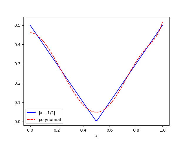
Let’s see how well we can approximate |x − ½| using prime exponents up to 11.
The polynomial above is
0.4605 − 5.233 x2 + 7.211 x3 + 0.9295 x5 − 4.4646 x7 + 1.614 x11.
This polynomial is not the best possible uniform approximation: it’s the least squares approximation. That is, it minimizes the 2-norm and not the ∞-norm. That’s because it’s convenient to do a least squares fit in Python using scipy.optimize.curve_fit.
Incidentally, the Müntz approximation theorem holds for the 2-norm as well.

